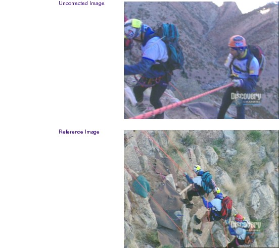
Analysis of original image: In this example, two different cameras have been used to shoot the rock climbers. The second camera is correctly balanced and shows good color characteristics. In comparison, the images from the first camera show a pronounced blue cast. Also, the image from the first camera is too dark. Because the images from the two cameras look so different from one another, and because the first image is intrinsically weak, corrections are needed to neutralize color and raise the brightness level in the first image. The image from the good camera can be used as a reference as these corrections are made. In this example, the corrections are made in the Curves tab. One advantage of Curves tab adjustments, if you are practiced and comfortable with them, is that you can make quite complex changes without having to alter many controls. The corrections in this example are made by adding and moving a single control point in each of two ChromaCurve graphs.

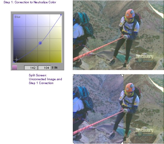
Step 1 of this correction removes the excess blue in the image by adjusting the Blue ChromaCurve graph in the Curves tab. A control point is placed near the center of the curve since the adjustment needs to apply relatively evenly across the whole luminance range. The control point is then dragged down to reduce blue. The input and output values for this adjustment are 142 and 104 respectively.

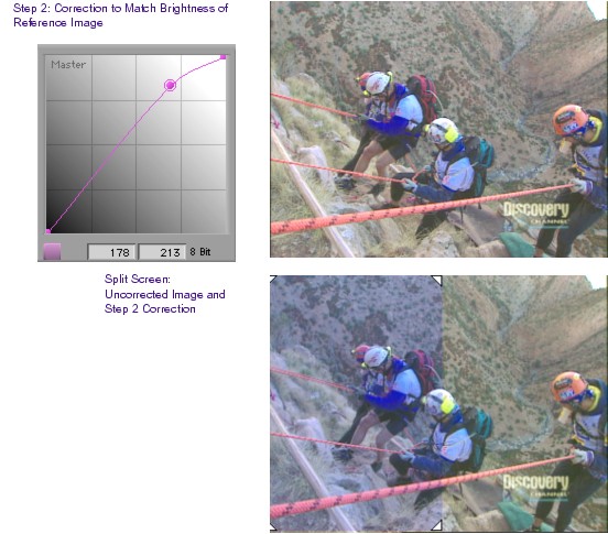
Step 2 of this correction increases the brightness of the image by making an adjustment on the Master ChromaCurve graph in the Curves tab. The control point is placed three-quarters of the way up the curve and moved up and to the left. The input and output values for this adjustment are 178 and 213 respectively. The resulting curve increases brightness throughout the image but increases it most in the highlights range. This creates more contrast in the lower three-quarters of the luminance range (in a ChromaCurve graph, contrast is greater where the curve is steeper).

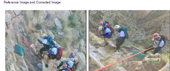
The following illustration compares the corrected image to the reference image from the good camera. Some fine-tuning is still possible to match the shots more precisely, but the images from the two cameras are now much closer to one another and will look more acceptable when viewed in the sequence.

Sample RGB values: A sample of one of the climber's white helmets before and after the correction and in the reference image shows the following values:

Though these samples might not be from precisely the same part of the helmet in all three cases, they clearly confirm the nature of the correction. They indicate a relative gain in red and green levels, a reduction in blue levels, and a much closer match with the levels in the reference frame.

Alternative techniques: The Blue ChromaCurve graph correction could be made in the Hue Offsets tab or even with a series of adjustments to the HSL sliders in the Controls tab. The brightness and contrast adjustment could be made in the HSL tab (using similar techniques to those in examples 1 and 2).